6. Smart Emission Project
NB The Smart Emission Project now (May 2016) has its own resources: website, GitHub etc. The info below is left here for historic reasons and not accurate anymore!! Please go to: www.smartemission.nl for all links to docs, GitHub etc
In september 2015 the SOSPilot platform was extended to handle air quality data from the Smart Emission (Nijmegen) project. The same ETL components and services (WMS, WFS, SOS) as used for RIVM AQ data were reused with some small modifications. Source code for the Smart Emission ETL can be found in GitHub: https://github.com/Geonovum/sospilot/tree/master/src/smartem . Small sample data used for development can be found at https://github.com/Geonovum/sospilot/tree/master/data/smartem
6.1. Background
Read about the Smart Emission project via: Smart Emission (Nijmegen) project. The figures below were taken from the Living Lab presentation, on June 24, 2015: http://www.ru.nl/publish/pages/774337/smartemission_ru_24juni_lc_v5_smallsize.pdf
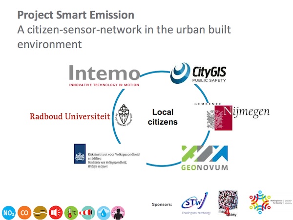
Smart Emission Project - Participants
In the paper Filling the feedback gap of place-related externalities in smart cities the project is described extensively.
”...we present the set-up of the pilot experiment in project “Smart Emission”, constructing an experimental citizen-sensor-network in the city of Nijmegen. This project, as part of research program ‘Maps 4 Society,’ is one of the currently running Smart City projects in the Netherlands. A number of social, technical and governmental innovations are put together in this project: (1) innovative sensing method: new, low-cost sensors are being designed and built in the project and tested in practice, using small sensing-modules that measure air quality indicators, amongst others NO2, CO2, ozone, temperature and noise load. (2) big data: the measured data forms a refined data-flow from sensing points at places where people live and work: thus forming a ‘big picture’ to build a real-time, in-depth understanding of the local distribution of urban air quality (3) empowering citizens by making visible the ‘externality’ of urban air quality and feeding this into a bottom-up planning process: the community in the target area get the co-decision-making control over where the sensors are placed, co-interpret the mapped feedback data, discuss and collectively explore possible options for improvement (supported by a Maptable instrument) to get a fair and ‘better’ distribution of air pollution in the city, balanced against other spatial qualities. ....”
The Sensor (Sensor Jose) used was developed by Intemo with Server-sensor connection by CityGIS. See below.
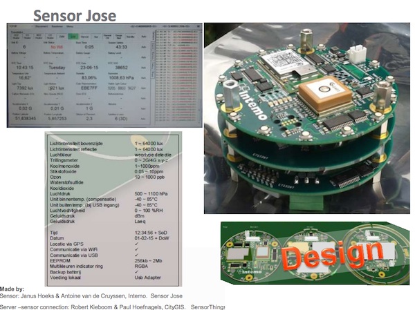
Smart Emission Project - Sensors
The data from these sensors was converted and published into standard OGC services: WMS(-Time), WFS and SOS. This is described in the remainder of this chapter. For readers eager to see the results, these are presented in the next section. A snapshot of AQ data was provided through CityGIS via FTP.
6.2. Results
Results can be viewed in basically 3 ways:
- as WMS and WMS-Time Layers via the Heron Viewer: http://sensors.geonovum.nl/heronviewer
- as SOS-data via the SOS Web-Client: http://sensors.geonovum.nl/jsclient
- as raw SOS-data via SOS or easier via the SOS-REST API
Below some guidance for each viewing method.
6.2.1. Heron Viewer
Within the Heron Viewer at http://sensors.geonovum.nl/heronviewer one can view Stations and Measurements. These are available as standard WMS layers organized as follows:
- Stations Layer: geo-locations and info of all stations (triangles)
- Last Measurements Layers: per-component Layers showing the last known measurements for each station
- Measurements History Layers: per-component Layers showing measurements over time for each station
To discern among RIVM LML and Smart Emission data, the latter Stations are rendered as pink-purple icons. The related measurements data (circles) have a pink-purple border.
6.2.1.1. Stations Layer
The figure below shows all stations from RIVM LML (orange active stations, grey inactive) and Smart Emission (pink-purple triangles).
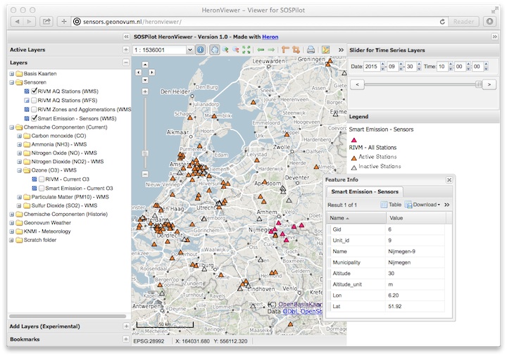
Smart Emission Stations in Heron Viewer
Clicking on a Station provides more detailed info via WMS GetFeatureInfo in a pop-up window.
6.2.1.2. Last Measurements Layers
In the viewer the latest measurements per station can be shown. NB the Smart Emission data may not be current. LML data is current, i.e. from the current last hour.
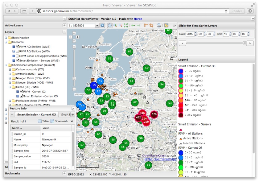
Heron Viewer showing latest known O3 Measurements
Use the map/folder on the left called “Chemische Componenten (Current)” to open a chemical component. For each component there are one or two (NO2, CO and O3) layers that can be enabled. Click on a circle to see more detail.
6.2.1.3. Measurements History Layers
This shows measurements through time (using WMS-Time). NB Smart Emission data is mainly from july/august 2015!
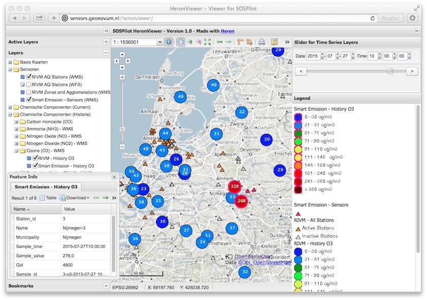
Heron Viewer showing O3 Measurements over time with timeslider
Use the map/folder on the left called “Chemische Componenten (Historie)”. For each component there are one or two (NO2, CO and O3)layers that can be enabled. Click on a circle to see more detail. Use the TimeSlider on the upper right to go through date and time. The image above shows O3 at July 27, 2015, 10:00. Pink-purple-bordered circles denote Smart Emission measurements.
6.2.2. SOS Web-Client
The SOS Web Client by 52North: http://sensors.geonovum.nl/jsclient accesses the SOS directly via the map and charts.
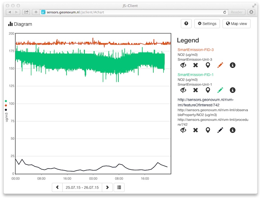
SOS Web Client showing NO2 Measurements in Chart
The viewer is quite advanced and
takes some time to get used to. It is possible to get charts and other views. Best is to follow
the built-in tutorial. Custom charts can be made by selecting stations on the map (Map View) and
adding these. The Smart Emission components are called O3, CO and NO2. The RIVM LML ones have
longer names starting with http:.
As can be seen the Smart Emission measurements are significantly higher. Also RIVM LML data is produced
as an hourly average while Smart Emission data (now) provides all measurements. This is an item for improvement.
6.2.3. SOS-REST API
Easiest is looking at results via the SOS REST API.
The following are examples:
- http://sensors.geonovum.nl/sos/api/v1/stations REST API, Stations
- http://sensors.geonovum.nl/sos/api/v1/phenomena REST API, Phenomena
- http://sensors.geonovum.nl/sos/api/v1/timeseries REST API, All Time Series List
- http://sensors.geonovum.nl/sos/api/v1/timeseries/260 REST API, Single Time Series MetaData
- http://sensors.geonovum.nl/sos/api/v1/timeseries/100/getData?timespan=PT48H/2014-09-06 REST API, Time Series Data
- http://sensors.geonovum.nl/sos/api/v1/timeseries/260/getData?timespan=2015-07-21TZ/2015-07-28TZ REST API, Time Series Data
The remainder of this chapter describes the technical setup.
6.3. Architecture
Figure 2 sketches the overall SOSPilot architecture with emphasis on the flow of data (arrows). Circles depict harvesting/ETL processes. Server-instances are in rectangles. Datastores the “DB”-icons.
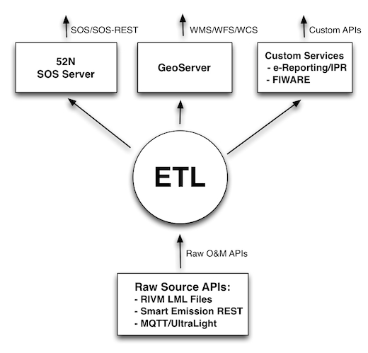
Figure 2 - Overall Architecture
Figure 2 sketches the approach for RIVM LML AQ data, but this same approach was used voor Smart Emission. For “RIVM LML File Server” one should read: “Raw Smart Emission Sample Data”.
6.4. ETL Design
In this section the ETL is elaborated in more detail as depicted in the figure below. Figure 3 sketches the same approach as earlier used for for RIVM LML AQ data. Step 1 and Step 2 are (partly) different from the RIVM LML ETL. Step 3 is identical to the RIVM LML ETL, an advantage of the multi-step ETL process now pays back! The main difference/extension to RIVM LML ETL processing is that the Smart Emission raw O&M data is not yet validated (e.g. has outliers) and aggregated (e.g. no hourly averages).
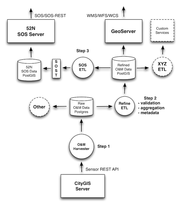
Figure 3 - Overall Architecture with ETL Steps
The ETL design comprises three main processing steps and three datastores. The three ETL Steps are:
- O&M Harvester: fetch raw O&M data from CityGIS server via Sensor REST API
- Refine ETL: validate and aggregate the raw O&M data and transform to intermediate “Core AQ Data” in PostGIS
- SOS ETL: transform and publish “Core AQ Data” to the 52N SOS DB via SOS-Transactions (SOS-T)
The detailed dataflow from source to destination is as follows:
- raw O&M timeseries data is read by the O&M Harvester via Sensor REST API
- O&M Harvester reads the timeseries response docs into the Raw O&M Data DB (Raw Measurements)
- The Core AQ DB contains measurements + stations in regular tables 1-1 with original data, including a Time column
- The Core AQ DB can be used for OWS (WMS/WFS) services via GeoServer (using VIEW by Measurements/Stations JOIN)
- The SOS ETL process transforms core AQ data to SOS Observations and publishes Observations using SOS-T
InsertObservation - These three processes run continuously (via cron)
- Each process always knows its progress and where it needs to resume, even after it has been stopped (by storing a progress/checkpoint info)
These last two ETL processes manage their last sync-time using a separate progress table within the database.
The first, the O&M Harvester, only needs to check if a particular timeseries for a specific device has already been stored.
Advantages of this approach:
- backups of source data possible
- incrementally build up of history past the last month
- in case of (design) errors we can always reset the ‘progress timestamp(s)’ and restart anew
- simpler ETL scripts than “all-in-one”, e.g. from “Core AQ DB” to “52N SOS DB” may even be in plain SQL
- migration with changed in 52N SOS DB schema simpler
- prepared for op IPR/INSPIRE ETL (source is Core OM DB)
- OWS server (WMS/WFS evt WCS) can directly use op Core OM DB (possibly via Measurements/Stations JOIN VIEW evt, see below)
The Open Source ETL tool Stetl, Streaming ETL , is used for most of the transformation steps. Stetl provides standard modules for building an ETL Chain via a configuration file. This ETL Chain is a linkage of Input, Filter and Output modules. Each module is a Python class derived from Stetl base classes. In addition a developer may add custom modules where standard Stetl modules are not available or to specialize processing aspects.
Stetl has been used sucessfully to publish BAG (Dutch Addresses and Buildings) to INSPIRE Addresses via
XSLT and WFS-T (to the deegree WFS server) but also for transformation of Dutch topography (Top10NL and BGT)
to PostGIS. As Stetl is written in Python it is well-integrated with standard ETL and Geo-tools like GDAl/OGR, XSLT and
PostGIS.
At runtime Stetl (via the stetl command) basically reads the config file,
creates all modules and links their inputs and outputs. This also makes for an easy programming model
as one only needs to concentrate on a single ETL step.
6.4.1. ETL Step 1. - Harvester
The Smart Emission FTP server provides measurements per sensor (unit) in text files. See figure below. The raw data records per unit are divided over multiple lines. See example below:
07/24/2015 07:25:41,P.UnitSerialnumber,1   # start record
07/24/2015 07:25:41,S.Longitude,5914103
07/24/2015 07:25:41,S.Latitude,53949942
07/24/2015 07:25:41,S.SatInfo,90889
07/24/2015 07:25:41,S.O3,163
07/24/2015 07:25:41,S.BottomSwitches,0
07/24/2015 07:25:41,S.RGBColor,16771990
07/24/2015 07:25:41,S.LightsensorBlue,92
07/24/2015 07:25:41,S.LightsensorGreen,144
07/24/2015 07:25:41,S.LightsensorRed,156
07/24/2015 07:25:41,S.AcceleroZ,753
07/24/2015 07:25:41,S.AcceleroY,516
07/24/2015 07:25:41,S.AcceleroX,510
07/24/2015 07:25:41,S.NO2,90
07/24/2015 07:25:41,S.CO,31755
07/24/2015 07:25:41,S.Altimeter,118
07/24/2015 07:25:41,S.Barometer,101101
07/24/2015 07:25:41,S.LightsensorBottom,26
07/24/2015 07:25:41,S.LightsensorTop,225
07/24/2015 07:25:41,S.Humidity,48618
07/24/2015 07:25:41,S.TemperatureAmbient,299425
07/24/2015 07:25:41,S.TemperatureUnit,305400
07/24/2015 07:25:41,S.SecondOfDay,33983
07/24/2015 07:25:41,S.RtcDate,1012101
07/24/2015 07:25:41,S.RtcTime,596503
07/24/2015 07:25:41,P.SessionUptime,60781
07/24/2015 07:25:41,P.BaseTimer,9
07/24/2015 07:25:41,P.ErrorStatus,0
07/24/2015 07:25:41,P.Powerstate,79
07/24/2015 07:25:51,P.UnitSerialnumber,1  # start record
07/24/2015 07:25:51,S.Longitude,5914103
07/24/2015 07:25:51,S.Latitude,53949942
07/24/2015 07:25:51,S.SatInfo,90889
07/24/2015 07:25:51,S.O3,157
07/24/2015 07:25:51,S.BottomSwitches,0
Each record starts on a line that contains P.UnitSerialnumber and runs to the next line
containing P.UnitSerialnumber or the end-of-file is reached. Each record contains
zero to three chemical component values named: S.CO (Carbon Monoxide), S.NO2 (Nitrogen Dioxide)
or S.O3 (Ozone), and further fields such as location (S.Latitude, S.Longitude) and
weather data (Temperature, Pressure). All fields have the same timestamp, e.g. 07/24/2015 07:25:41.
This value is taken as the timestamp of the record.
According to CityGIS the units are defined as follows.
S.TemperatureUnit            milliKelvin
S.TemperatureAmbient milliKelvin
S.Humidity                           %mRH
S.LightsensorTop             Lux
S.LightsensorBottom          Lux
S.Barometer                          Pascal
S.Altimeter                          Meter
S.CO                                 ppb
S.NO2                                        ppb
S.AcceleroX                          2 ~ +2G (0x200 = midscale)
S.AcceleroY                          2 ~ +2G (0x200 = midscale)
S.AcceleroZ                          2 ~ +2G (0x200 = midscale)
S.LightsensorRed             Lux
S.LightsensorGreen           Lux
S.LightsensorBlue            Lux
S.RGBColor                           8 bit R, 8 bit G, 8 bit B
S.BottomSwitches             ?
S.O3                                 ppb
S.CO2                                        ppb
v3: S.ExternalTemp           milliKelvin
v3: S.COResistance           Ohm
v3: S.No2Resistance          Ohm
v3: S.O3Resistance           Ohm
S.AudioMinus5                        Octave -5 in dB(A)
S.AudioMinus4                        Octave -4 in dB(A)
S.AudioMinus3                        Octave -3 in dB(A)
S.AudioMinus2                        Octave -2 in dB(A)
S.AudioMinus1                        Octave -1 in dB(A)
S.Audio0                             Octave 0 in dB(A)
S.AudioPlus1                 Octave +1 in dB(A)
S.AudioPlus2                 Octave +2 in dB(A)
S.AudioPlus3                 Octave +3 in dB(A)
S.AudioPlus4                 Octave +4 in dB(A)
S.AudioPlus5                 Octave +5 in dB(A)
S.AudioPlus6                 Octave +6 in dB(A)
S.AudioPlus7                 Octave +7 in dB(A)
S.AudioPlus8                 Octave +8 in dB(A)
S.AudioPlus9                 Octave +9 in dB(A)
S.AudioPlus10                        Octave +10 in dB(A)
S.SatInfo
S.Latitude                           nibbles: n1:0=East/North, 8=West/South; n2&n3: whole degrees (0-180); n4-n8: degree fraction (max 999999)
S.Longitude                          nibbles: n1:0=East/North, 8=West/South; n2&n3: whole degrees (0-180); n4-n8: degree fraction (max 999999)

P.Powerstate                                 Power State
P.BatteryVoltage                             Battery Voltage (milliVolts)
P.BatteryTemperature                 Battery Temperature (milliKelvin)
P.BatteryGauge                                       Get Battery Gauge, BFFF = Battery full, 1FFF = Battery fail, 0000 = No Battery Installed
P.MuxStatus                                          Mux Status (0-7=channel,F=inhibited)
P.ErrorStatus                                        Error Status (0=OK)
P.BaseTimer                                          BaseTimer (seconds)
P.SessionUptime                                      Session Uptime (seconds)
P.TotalUptime                                        Total Uptime (minutes)
v3: P.COHeaterMode                           CO heater mode
P.COHeater                                           Powerstate CO heater (0/1)
P.NO2Heater                                          Powerstate NO2 heater (0/1)
P.O3Heater                                           Powerstate O3 heater (0/1)
v3: P.CO2Heater                                      Powerstate CO2 heater (0/1)
P.UnitSerialnumber                           Serialnumber of unit
P.TemporarilyEnableDebugLeds Debug leds (0/1)
P.TemporarilyEnableBaseTimer Enable BaseTime (0/1)
P.ControllerReset                            WIFI reset
P.FirmwareUpdate                             Firmware update, reboot to bootloader

Unknown at this moment (decimal):
P.11
P.16
P.17
P.18
Conversion for latitude/longitude:
/*
            8 nibbles:
            MSB                  LSB
            n1 n2 n3 n4 n5 n6 n7 n8
            n1: 0 of 8, 0=East/North, 8=West/South
            n2 en n3: whole degrees (0-180)
            n4-n8: fraction of degrees (max 999999)
*/
private convert(input: number): number {
    var sign = input >> 28 ? -1 : +1;
    var deg = (input >> 20) & 255;
    var dec = input & 1048575;

    return (deg + dec / 1000000) * sign;
}
As stated above: this step, acquiring/harvesting files, was initially done via FTP.
6.4.2. ETL Step 2 - Raw Measurements
This step produces raw AQ measurements, “AQ ETL” in Figure 2, from raw source (file) data harvested in Step 1. The results of this step can be accessed via WMS and WFS, directly in the project Heron viewer: http://sensors.geonovum.nl/heronviewer
Two tables: stations and measurements. This is a 1:1 transformation from the raw text.
The measurements refers to the stations by a FK unit_id.
6.4.2.1. Stations
Station info has been assembled in a CSV file: https://github.com/Geonovum/sospilot/tree/master/src/smartem/stations.csv
UnitId,Name,Municipality,Lat,Lon,Altitude,AltitudeUnit
1,Nijmegen-1,Nijmegen,51.94,5.90,30,m
3,Nijmegen-3,Nijmegen,51.80,6.00,30,m
5,Nijmegen-5,Nijmegen,51.85,5.95,30,m
7,Nijmegen-7,Nijmegen,51.91,6.10,30,m
8,Nijmegen-8,Nijmegen,51.87,5.80,30,m
9,Nijmegen-9,Nijmegen,51.92,6.20,30,m
10,Nijmegen-10,Nijmegen,51.89,5.85,30,m
This info was deducted from the raw measurements files. NB: the Lat,Lon values were inaccurate. This is still under investigation. For the sake of the project Lat,Lon values have been randomly altered here!. This will need to be corrected at a later stage.
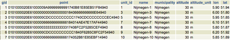
Stations Read into Postgres/PostGIS
Test by viewing in http://sensors.geonovum.nl/heronviewer
See result (pink-purple triangles). Clicking on a station provides more detailed info via WMS GetFeatureInfo.
Smart Emission Stations in Heron Viewer
6.4.2.2. Measurements
Reading raw measurements from the files is done with a Stetl
process. A specific Stetl Input module was developed to effect reading and parsing the files
and tracking the last id of the file processed.
https://github.com/Geonovum/sospilot/blob/master/src/smartem/raw2measurements.py
These are two Filters: the class Raw2RecordFilter converts raw lines from the
file to raw records. The class Record2MeasurementsFilter converts these records to
records to be inserted into the measurements table. Other components used are standard Stetl.
Unit Conversion: as seen above the units for chemical components are in ppb (Parts-Per-Billion).
For AQ data the usual unit is ug/m3 (Microgram per cubic meter). The conversion
from ppb to ug/m3 is well-known and is dependent on molecular weight, temperature
and pressure. See more detail here: http://www.apis.ac.uk/unit-conversion. Some investigation:
# Zie http://www.apis.ac.uk/unit-conversion
# ug/m3 = PPB * moleculair gewicht/moleculair volume
# waar molec vol = 22.41 * T/273 * 1013/P
#
# Typical values:
# Nitrogen dioxide 1 ppb = 1.91 ug/m3  bij 10C 1.98, bij 30C 1.85 --> 1.9
# Ozone 1 ppb = 2.0 ug/m3  bij 10C 2.1, bij 30C 1.93 --> 2.0
# Carbon monoxide 1 ppb = 1.16 ug/m3 bij 10C 1.2, bij 30C 1.1 --> 1.15
#
# Benzene 1 ppb = 3.24 ug/m3
# Sulphur dioxide 1 ppb = 2.66 ug/m3
#
For now a crude approximation as the measurements themselves are also not very accurate (another issue). In raw2measurements.py:
record['sample_value'] = Record2MeasurementsFilter.ppb_to_ugm3_factor[component_name] * ppb_val
with Record2MeasurementsFilter.ppb_to_ugm3_factor:
# For now a crude conversion (1 atm, 20C)
ppb_to_ugm3_factor = {'o3': 2.0, 'no2': 1.9, 'co': 1.15}
The entire Stetl process is defined in https://github.com/Geonovum/sospilot/blob/master/src/smartem/files2measurements.cfg
The invokation of that Stetl process is via shell script: https://github.com/Geonovum/sospilot/blob/master/src/smartem/files2measurements.sh
The data is stored in the measurements table, as below. station_id is a foreign key
into the stations table corresponding to a unit_id.
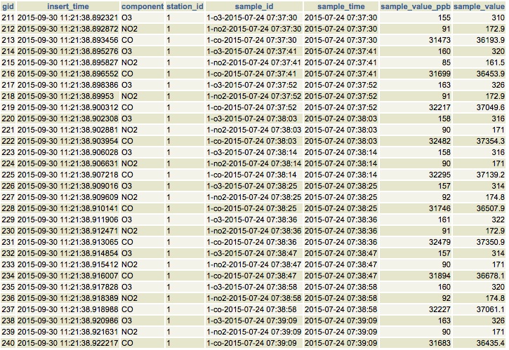
Smart Emission raw measurements stored in Postgres
Using a Postgres VIEW the two tables can be combined via an INNER JOIN to provide measurements
with location. This VIEW can be used as a WMS/WFS data source in GeoServer.
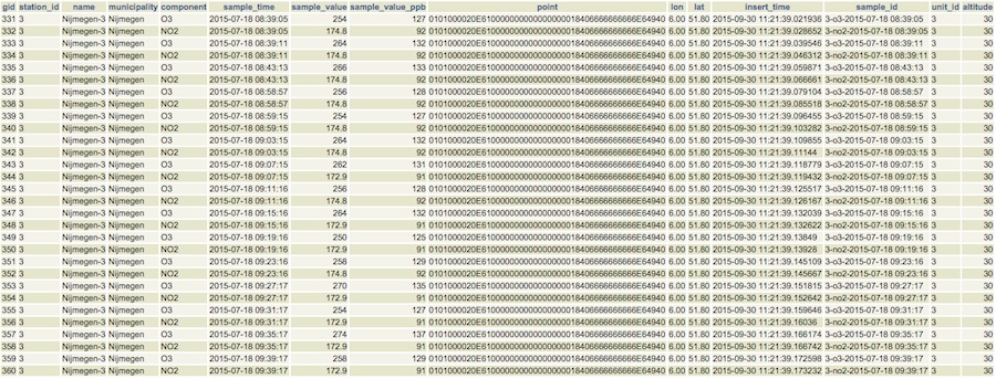
Postgres VIEW combining measurements and stations (units)
The VIEW is defined in https://github.com/Geonovum/sospilot/blob/master/src/smartem/db/db-schema.sql:
CREATE VIEW smartem.measurements_stations AS
   SELECT m.gid, m.station_id, s.name, s.municipality, m.component, m.sample_time, m.sample_value,
   m.sample_value_ppb, s.point, s.lon, s.lat,m.insert_time, m.sample_id,s.unit_id, s.altitude
          FROM smartem.measurements as m
            INNER JOIN smartem.stations as s ON m.station_id = s.unit_id;
Other detailed VIEWs provide virtual tables like Last Measurements and Measurements per component (see the DB schema and the Heron viewer).
6.4.3. ETL Step 3 - SOS Publication
In this step the Raw Measurements data (see Step 2) is transformed to “SOS Ready Data”,
i.e. data that can be handled by the 52North SOS server. This is done via
SOS Transaction (SOS-T) services using Stetl.
6.4.3.1. SOS Publication - Stetl Strategy
As Stetl only supports WFS-T, not yet SOS, a SOS Output module sosoutput.py was developed derived
from the standard httpoutput.py module.
See https://github.com/Geonovum/sospilot/blob/master/src/smartem/sosoutput.py (this version was slightly
adapted from the version used for RIVM LML).
Most importantly, the raw Smart Emission Measurements data
from Step 2 needs to be transformed to OWS Observations & Measurements (O&M) data. This is done via substitutable templates, like the
Stetl config itself also applies. This means we develop files with SOS Requests in which all variable parts get a
symbolic value like {sample_value}. These templates can be found under
https://github.com/Geonovum/sospilot/tree/master/src/smartem/sostemplates in particular
- https://github.com/Geonovum/sospilot/blob/master/src/smartem/sostemplates/insert-sensor.json InsertSensor
- https://github.com/Geonovum/sospilot/blob/master/src/smartem/sostemplates/delete-sensor.json DeleteSensor
- https://github.com/Geonovum/sospilot/blob/master/src/smartem/sostemplates/procedure-desc.xml Sensor ML
- https://github.com/Geonovum/sospilot/blob/master/src/smartem/sostemplates/insert-observation.json InsertObservation
Note that we use JSON for the requests, as this is simpler than XML. The Sensor ML is embedded in the
insert-sensor JSON request.
6.4.3.2. SOS Publication - Sensors
This step needs to be performed only once, or when any of the original Station data (CSV) changes.
The Stetl config https://github.com/Geonovum/sospilot/blob/master/src/smartem/stations2sensors.cfg
uses a Standard Stetl module, inputs.dbinput.PostgresDbInput for obtaining Record data from a Postgres database.
{{
  "request": "InsertSensor",
  "service": "SOS",
  "version": "2.0.0",
  "procedureDescriptionFormat": "http://www.opengis.net/sensorML/1.0.1",
  "procedureDescription": "{procedure-desc.xml}",
   "observableProperty": [
    "CO",
    "NO2",
    "O3"
  ],
  "observationType": [
    "http://www.opengis.net/def/observationType/OGC-OM/2.0/OM_Measurement"
  ],
  "featureOfInterestType": "http://www.opengis.net/def/samplingFeatureType/OGC-OM/2.0/SF_SamplingPoint"
}}
The SOSTOutput module will expand {procedure-desc.xml} with the Sensor ML template from
https://github.com/Geonovum/sospilot/blob/master/src/smartem/sostemplates/procedure-desc.xml.
6.4.3.3. SOS Publication - Observations
The Stetl config https://github.com/Geonovum/sospilot/blob/master/src/smartem/measurements2sos.cfg
uses an extended Stetl module (inputs.dbinput.PostgresDbInput) for obtaining Record data from a Postgres database:
https://github.com/Geonovum/sospilot/blob/master/src/smartem/measurementsdbinput.py.
This is required to track progress in the etl_progress table similar as in Step 2.
The last_id is remembered.
The Observation template looks as follows.
{{
  "request": "InsertObservation",
  "service": "SOS",
  "version": "2.0.0",
  "offering": "SmartEmission-Offering-{unit_id}",
  "observation": {{
    "identifier": {{
      "value": "{sample_id}",
      "codespace": "http://www.opengis.net/def/nil/OGC/0/unknown"
    }},
    "type": "http://www.opengis.net/def/observationType/OGC-OM/2.0/OM_Measurement",
    "procedure": "SmartEmission-Unit-{unit_id}",
    "observedProperty": "{component}",
    "featureOfInterest": {{
      "identifier": {{
        "value": "SmartEmission-FID-{unit_id}",
        "codespace": "http://www.opengis.net/def/nil/OGC/0/unknown"
      }},
      "name": [
        {{
          "value": "{municipality}",
          "codespace": "http://www.opengis.net/def/nil/OGC/0/unknown"
        }}
      ],
      "geometry": {{
        "type": "Point",
        "coordinates": [
          {lat},
          {lon}
        ],
        "crs": {{
          "type": "name",
          "properties": {{
            "name": "EPSG:4326"
          }}
        }}
      }}
    }},
    "phenomenonTime": "{sample_time}",
    "resultTime": "{sample_time}",
    "result": {{
      "uom": "ug/m3",
      "value": {sample_value}
    }}
  }}
}}
It is quite trivial in sosoutput.py to substitute these values from the measurements-table records.
Like in ETL Step 2 the progress is remembered in the table rivm_lml.etl_progress by updating the last_id field
after publication, where that value represents the gid value of rivm_lml.measurements.
6.4.3.4. SOS Publication - Results
Via the standard SOS protocol the results can be tested:
- GetCapabilities: http://sensors.geonovum.nl/sos/service?service=SOS&request=GetCapabilities
- DescribeSensor (station 807, Hellendoorn): http://tinyurl.com/mmsr9hl (URL shortened)
- GetObservation: http://tinyurl.com/ol82sxv (URL shortened)
Easier is looking at results via the SOS REST API. The following are examples:
- http://sensors.geonovum.nl/sos/api/v1/stations REST API, Stations
- http://sensors.geonovum.nl/sos/api/v1/phenomena REST API, Phenomena
- http://sensors.geonovum.nl/sos/api/v1/timeseries REST API, All Time Series List
- http://sensors.geonovum.nl/sos/api/v1/timeseries/260 REST API, Single Time Series MetaData
- http://sensors.geonovum.nl/sos/api/v1/timeseries/100/getData?timespan=PT48H/2014-09-06 REST API, Time Series Data
- http://sensors.geonovum.nl/sos/api/v1/timeseries/260/getData?timespan=2015-07-21TZ/2015-07-28TZ REST API, Time Series Data